Hands On: ksqlDB

Hands On: ksqIDB

In this exercise, you’ll learn how to manipulate your data using ksqlDB. Up until now, we’ve been producing data to and reading data from an Apache Kafka topic without any intermediate steps. With data transformation and aggregation, we can do so much more!

In the last exercise, we created a Datagen Source Connector to produce a stream of orders data to a Kafka topic, serializing it in Avro using Confluent Schema Registry along the way. This exercise relies on the data that our connector is producing, so if you haven’t completed the previous exercise, we encourage you to do so beforehand.

Before we start, make sure that your Datagen Source Connector is still up and running.

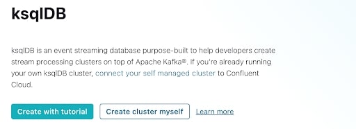
1. From the cluster landing page in the Confluent Cloud Console, select ksqlDB from the left-hand menu. Select Create cluster myself.

   

2. Choose Global access from the “Access Control” page; select Continue to give the ksqlDB cluster a name and then Launch cluster. When the ksqlDB cluster is finished provisioning, you’ll be taken to the ksqlDB editor. From this UI, you can enter SQL statements to access, aggregate, and transform your data.

3. Add the orders topic from the previous exercise to the ksqlDB application. Register it as a stream by running:

   CREATE STREAM orders_stream WITH (
     KAFKA_TOPIC='orders', 
     VALUE_FORMAT='AVRO',
     PARTITIONS=6,
     TIMESTAMP='ordertime');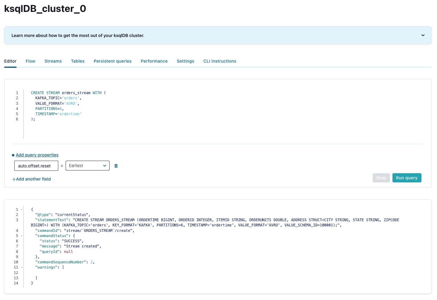

   

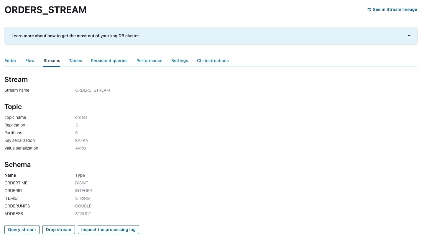
4. When the stream has been created, navigate to the Streams tab and select the orders_stream to view more details about the stream, including fields and their types, how the data is serialized, and information about the underlying topic.

   

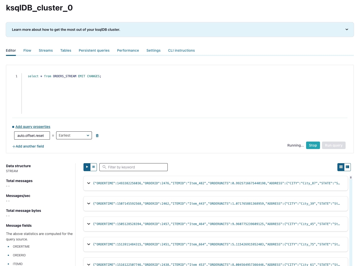
5. Click Query stream to be taken directly back to the editor, where the editor will be automatically populated with a query for that stream of data. If your Datagen connector is still running (which it should be), you’ll also see data being output in real time at the bottom of the screen.

   

6. The ordertime field of each message is in milliseconds since epoch, which isn’t very friendly to look at. To transform this field into something more readable, execute the following push query (which will output results as new messages are written to the underlying Kafka topic):

   SELECT 
       TIMESTAMPTOSTRING(ORDERTIME, 'yyyy-MM-dd HH:mm:ss.SSS') AS ORDERTIME_FORMATTED,
       orderid,
       itemid,
       orderunits,
       address->city, 
       address->state,
       address->zipcode
   from ORDERS_STREAM;

   This query also extracts the nested data from the address struct.

7. The results look good, so add a CREATE STREAM line to the beginning of the query to persist the results to a new stream.

   CREATE STREAM ORDERS_STREAM_TS AS
   SELECT 
       TIMESTAMPTOSTRING(ORDERTIME, 'yyyy-MM-dd HH:mm:ss.SSS') AS ORDERTIME_FORMATTED,
       orderid,
       itemid,
       orderunits,
       address->city, 
       address->state,
       address->zipcode 
   from ORDERS_STREAM;

8. Using data aggregations, you can determine how many orders are made per state. ksqlDB also makes it easy to window data so that you can easily determine how many orders are made per state per week. Run the following ksqlDB statement to create a table:

   CREATE TABLE STATE_COUNTS AS 
   SELECT 
     address->state,
     COUNT_DISTINCT(ORDERID) AS DISTINCT_ORDERS
   FROM ORDERS_STREAM
   WINDOW TUMBLING (SIZE 7 DAYS) 
   GROUP BY address->state;

9. When the table has been created, navigate to the Tables tab above to see data related to the table.

10. Click Query table to be taken back to the ksqlDB editor and start an open-ended query that will provide an output for each update to the table; as new orders are made, you’ll see an ever-increasing number of orders per state per defined window period.

11. In order to just see the latest values from a table—rather than an open-ended query—we can execute a pull query. We can see a current snapshot containing the states that had over two orders per one-week period by running the following:

    SELECT
        *
    FROM STATE_COUNTS
    WHERE DISTINCT_ORDERS > 2;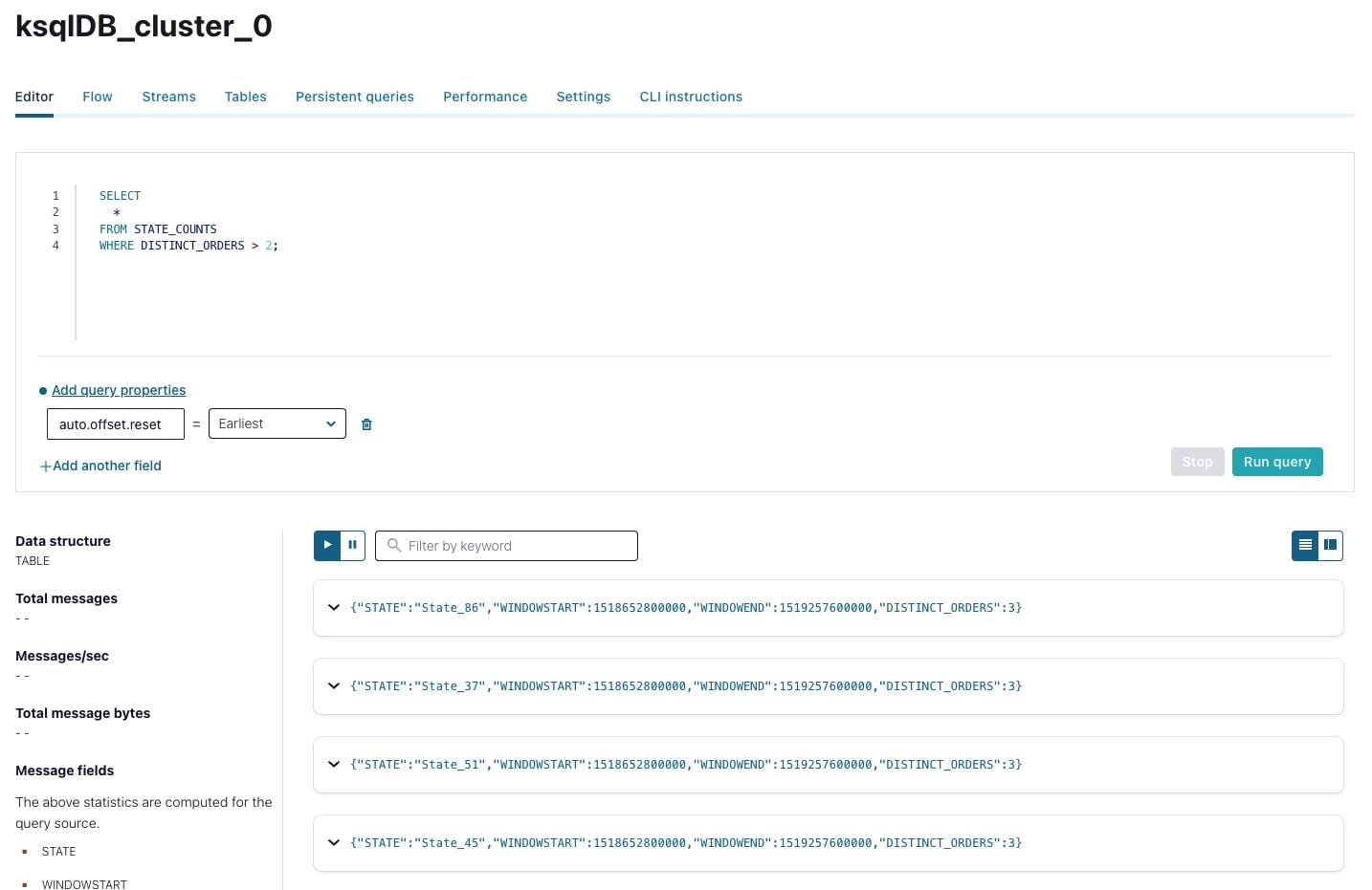

    

We've only scratched the surface of what you can do with ksqlDB, but we’ve shown you how to create streams and tables as well as how to transform and aggregate your data. With these tools in your toolbelt, you’ll be able to hit the ground running with your next ksqlDB application. If you’d like to learn about ksqlDB in more depth, definitely check out the ksqlDB 101 and Inside ksqlDB courses.